
Professional Data Engineer - Google Cloud Certified Exam Questions
Total Questions
Last Updated
1st Try Guaranteed

Experts Verified
Question 11 Single Choice
At WeatherSense Labs, you're developing a machine learning model to predict rainfall for a given day. Your dataset contains thousands of input features, and you want to explore ways to speed up model training while keeping the impact on accuracy minimal.
What approach should you consider?
Explanation

Click "Show Answer" to see the explanation here
B. Merge features that are highly interdependent into a single representative feature
Reducing thousands of raw inputs to a smaller set of composite or “aggregated” features (for example, by combining strongly correlated variables or by applying dimensionality-reduction techniques such as PCA) shrinks the feature space that the optimisation algorithm must traverse. Fewer features mean fewer parameters, faster forward/back-prop passes, and quicker convergence—often with little or no loss in accuracy because the merged feature still captures most of the original information. Encord | GeeksforGeeks
Why the other options are less suitable
A – Remove features strongly correlated with the target label
Those features are usually the most predictive; dropping them is likely to hurt accuracy more than it helps speed.C – Average every three features
Arbitrary grouping can discard signal and introduce noise, often harming accuracy without any principled gain in efficiency.D – Drop features with > 50 % nulls
Eliminating very sparse columns can be worthwhile, but the 50 % rule of thumb is heuristic; useful but incomplete. It does not directly address the many still-present, highly correlated features that dominate training time.
Merging or otherwise compressing interdependent features tackles the root cause—high dimensionality—while keeping most of the predictive power, delivering the greatest speed-up for minimal accuracy impact.
Explanation
B. Merge features that are highly interdependent into a single representative feature
Reducing thousands of raw inputs to a smaller set of composite or “aggregated” features (for example, by combining strongly correlated variables or by applying dimensionality-reduction techniques such as PCA) shrinks the feature space that the optimisation algorithm must traverse. Fewer features mean fewer parameters, faster forward/back-prop passes, and quicker convergence—often with little or no loss in accuracy because the merged feature still captures most of the original information. Encord | GeeksforGeeks
Why the other options are less suitable
A – Remove features strongly correlated with the target label
Those features are usually the most predictive; dropping them is likely to hurt accuracy more than it helps speed.C – Average every three features
Arbitrary grouping can discard signal and introduce noise, often harming accuracy without any principled gain in efficiency.D – Drop features with > 50 % nulls
Eliminating very sparse columns can be worthwhile, but the 50 % rule of thumb is heuristic; useful but incomplete. It does not directly address the many still-present, highly correlated features that dominate training time.
Merging or otherwise compressing interdependent features tackles the root cause—high dimensionality—while keeping most of the predictive power, delivering the greatest speed-up for minimal accuracy impact.
Question 12 Single Choice
NovaTech Manufacturing is streaming real-time sensor data from its production floor into Cloud Bigtable. However, the team has observed severe performance issues, particularly with queries used to power real-time dashboards.
To improve query performance, how should the row key design be modified?
Explanation
Click "Show Answer" to see the explanation here
Correct Answer: D. Use a row key structured as <sensor_id>#<timestamp>
✅ Justification for Correct Option (D)
Cloud Bigtable stores rows lexicographically sorted by row key, and row key design is critical for performance, especially for querying time-series sensor data.
Using a row key in the format: <sensor_id>#<timestamp>
offers the following benefits:
Efficient scans for a given sensor: You can easily retrieve all data for a single sensor by prefix-scanning with
sensor_id.Maintains time-ordering within each sensor’s data stream.
Enables efficient dashboard queries that typically look up data for one or more sensors within a time range.
Avoids hotspotting by naturally distributing rows if sensor IDs are diverse.
📚 Reference:
❌ Why the Other Options Are Incorrect
A. <timestamp>
Results in severe hotspotting because all incoming writes for the same time window target the same tablet node.
Poor distribution across nodes.
Not optimized for querying per sensor.
B. <sensor_id>
Lacks temporal ordering, so cannot efficiently scan recent events.
Not suitable for time-series queries like "last 10 minutes of data for sensor A".
Cannot efficiently filter by time range.
C. <timestamp>#<sensor_id>
Also leads to hotspotting, similar to Option A.
Primary sort order is by timestamp, which concentrates writes at the "tail".
Inefficient for queries by sensor.
✅ Summary
To optimize Cloud Bigtable for real-time dashboard queries of sensor data, design your row keys as:
→ <sensor_id>#<timestamp> (Option D)
This provides fast, scalable, and time-ordered access to per-sensor data without causing performance bottlenecks.
Explanation
Correct Answer: D. Use a row key structured as <sensor_id>#<timestamp>
✅ Justification for Correct Option (D)
Cloud Bigtable stores rows lexicographically sorted by row key, and row key design is critical for performance, especially for querying time-series sensor data.
Using a row key in the format: <sensor_id>#<timestamp>
offers the following benefits:
Efficient scans for a given sensor: You can easily retrieve all data for a single sensor by prefix-scanning with
sensor_id.Maintains time-ordering within each sensor’s data stream.
Enables efficient dashboard queries that typically look up data for one or more sensors within a time range.
Avoids hotspotting by naturally distributing rows if sensor IDs are diverse.
📚 Reference:
❌ Why the Other Options Are Incorrect
A. <timestamp>
Results in severe hotspotting because all incoming writes for the same time window target the same tablet node.
Poor distribution across nodes.
Not optimized for querying per sensor.
B. <sensor_id>
Lacks temporal ordering, so cannot efficiently scan recent events.
Not suitable for time-series queries like "last 10 minutes of data for sensor A".
Cannot efficiently filter by time range.
C. <timestamp>#<sensor_id>
Also leads to hotspotting, similar to Option A.
Primary sort order is by timestamp, which concentrates writes at the "tail".
Inefficient for queries by sensor.
✅ Summary
To optimize Cloud Bigtable for real-time dashboard queries of sensor data, design your row keys as:
→ <sensor_id>#<timestamp> (Option D)
This provides fast, scalable, and time-ordered access to per-sensor data without causing performance bottlenecks.
Question 13 Single Choice
You’re building a clothing recommendation system at StyleSense AI, which must adapt to changing fashion trends and user preferences over time. You've already implemented a streaming data pipeline that delivers new interaction data to the model as it becomes available.
How should you incorporate this new data into your model training strategy?
Explanation
Click "Show Answer" to see the explanation here
The correct answer is:
B. Continuously retrain the model using a combination of historical and new data.
Correct Option Explanation
B. Continuously retrain the model using a combination of historical and new data
Why it’s correct:
In recommendation systems that must adapt to dynamic patterns like changing fashion trends and user preferences, it’s critical to continuously retrain the model.
Using only new data (Option A) can cause the model to forget past patterns and lead to data drift or catastrophic forgetting.
Combining historical data with new streaming data ensures:
The model retains knowledge of long-term trends
While adapting to recent behavior
Leads to better generalization and user experience
This is especially important in domains like fashion where seasonal patterns and recency matter, but past trends still carry value.
Best Practices Reference:
Incorrect Option Justifications
A. Continuously retrain the model using only the new data
Why it’s incorrect:
This can lead to overfitting to recent data and loss of important historical patterns.
Makes the model unstable and prone to concept drift without context from the past.
C. Use the existing data for training, and treat the new data as the test set
Why it’s incorrect:
This approach does not incorporate the new data into training, which is essential for up-to-date recommendations.
New data is wasted as a test set instead of used to improve model adaptability.
D. Train the model using new data, and use the existing data as the test set
Why it’s incorrect:
Using older data as a test set for a model trained only on new data violates proper evaluation practices.
Test data should be representative of future data, not the past.
Also, training only on new data misses valuable long-term user patterns.
Conclusion:
For adaptive, real-time systems like clothing recommenders at StyleSense AI, the best practice is to retrain models with both historical and new data to ensure stability, adaptability, and accuracy over time.
Explanation
The correct answer is:
B. Continuously retrain the model using a combination of historical and new data.
Correct Option Explanation
B. Continuously retrain the model using a combination of historical and new data
Why it’s correct:
In recommendation systems that must adapt to dynamic patterns like changing fashion trends and user preferences, it’s critical to continuously retrain the model.
Using only new data (Option A) can cause the model to forget past patterns and lead to data drift or catastrophic forgetting.
Combining historical data with new streaming data ensures:
The model retains knowledge of long-term trends
While adapting to recent behavior
Leads to better generalization and user experience
This is especially important in domains like fashion where seasonal patterns and recency matter, but past trends still carry value.
Best Practices Reference:
Incorrect Option Justifications
A. Continuously retrain the model using only the new data
Why it’s incorrect:
This can lead to overfitting to recent data and loss of important historical patterns.
Makes the model unstable and prone to concept drift without context from the past.
C. Use the existing data for training, and treat the new data as the test set
Why it’s incorrect:
This approach does not incorporate the new data into training, which is essential for up-to-date recommendations.
New data is wasted as a test set instead of used to improve model adaptability.
D. Train the model using new data, and use the existing data as the test set
Why it’s incorrect:
Using older data as a test set for a model trained only on new data violates proper evaluation practices.
Test data should be representative of future data, not the past.
Also, training only on new data misses valuable long-term user patterns.
Conclusion:
For adaptive, real-time systems like clothing recommenders at StyleSense AI, the best practice is to retrain models with both historical and new data to ensure stability, adaptability, and accuracy over time.
Question 14 Single Choice
At DataVista Corp, you've built a critical dashboard in Looker Studio 360 (formerly Google Data Studio) for your large internal team. The dashboard pulls data from BigQuery as its source. However, you've observed that the visualizations are not displaying data generated within the last hour.
What should you do to resolve this and ensure the dashboard shows the most up-to-date data?
Explanation
Click "Show Answer" to see the explanation here
The correct answer is:
A. Turn off data caching by modifying the report settings in Looker Studio.
Correct Option Explanation
A. Turn off data caching by modifying the report settings in Looker Studio
Why it’s correct:
Looker Studio 360 (formerly Google Data Studio) uses data caching to improve performance and reduce the number of queries sent to BigQuery.
By default, Looker Studio may cache data for up to 12 hours, meaning recent data (like data from the last hour) might not appear in visualizations.
You can resolve this by turning off or modifying the data freshness settings in the report:
Go to Resource > Manage added data sources > Edit.
In the BigQuery connector settings, find the “Caching” options.
Set “Data freshness” to a lower value (e.g., 15 minutes) or disable caching entirely.
This ensures that every time the dashboard loads, it pulls the latest data directly from BigQuery.
Official Documentation:
Incorrect Option Justifications
B. Disable caching settings directly in the BigQuery table configuration
Why it’s incorrect:
BigQuery itself doesn’t cache table data in a way that affects Looker Studio dashboard freshness.
Caching is managed in Looker Studio, not in the BigQuery table configuration.
C. Refresh your browser tab that displays the dashboard
Why it’s incorrect:
Refreshing the tab only reloads the report from Looker Studio’s cache, unless the data freshness setting has been lowered.
It won’t bypass Looker Studio's internal cache, so recent data still won’t appear.
D. Clear your browser history from the last hour and reload the dashboard
Why it’s incorrect:
Browser history/cache has no impact on Looker Studio’s data freshness or query behavior.
The issue is entirely related to server-side caching in Looker Studio, not client-side caching.
Conclusion:
To ensure your dashboard always shows the latest data, control the caching behavior directly in Looker Studio's data source settings.
Explanation
The correct answer is:
A. Turn off data caching by modifying the report settings in Looker Studio.
Correct Option Explanation
A. Turn off data caching by modifying the report settings in Looker Studio
Why it’s correct:
Looker Studio 360 (formerly Google Data Studio) uses data caching to improve performance and reduce the number of queries sent to BigQuery.
By default, Looker Studio may cache data for up to 12 hours, meaning recent data (like data from the last hour) might not appear in visualizations.
You can resolve this by turning off or modifying the data freshness settings in the report:
Go to Resource > Manage added data sources > Edit.
In the BigQuery connector settings, find the “Caching” options.
Set “Data freshness” to a lower value (e.g., 15 minutes) or disable caching entirely.
This ensures that every time the dashboard loads, it pulls the latest data directly from BigQuery.
Official Documentation:
Incorrect Option Justifications
B. Disable caching settings directly in the BigQuery table configuration
Why it’s incorrect:
BigQuery itself doesn’t cache table data in a way that affects Looker Studio dashboard freshness.
Caching is managed in Looker Studio, not in the BigQuery table configuration.
C. Refresh your browser tab that displays the dashboard
Why it’s incorrect:
Refreshing the tab only reloads the report from Looker Studio’s cache, unless the data freshness setting has been lowered.
It won’t bypass Looker Studio's internal cache, so recent data still won’t appear.
D. Clear your browser history from the last hour and reload the dashboard
Why it’s incorrect:
Browser history/cache has no impact on Looker Studio’s data freshness or query behavior.
The issue is entirely related to server-side caching in Looker Studio, not client-side caching.
Conclusion:
To ensure your dashboard always shows the latest data, control the caching behavior directly in Looker Studio's data source settings.
Question 15 Single Choice
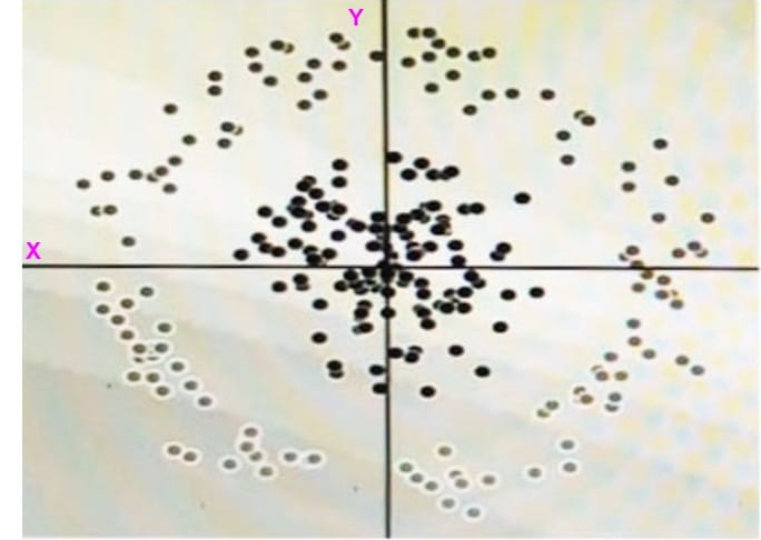
You have a dataset with two dimensions, X and Y, and each data point is shaded to represent its class. To accurately classify this data using a linear algorithm, you plan to introduce a synthetic feature. What should be the value of that feature?
Explanation
Click "Show Answer" to see the explanation here
Option A (X² + Y²) is indeed the most suitable choice for introducing a synthetic feature in this scenario. Here's a comprehensive explanation along with why other options might not be ideal:
Why X² + Y² is a Good Choice:
Enhancing Separability: Imagine the data points form a non-linear pattern in the X-Y plane, making linear separation difficult. X² + Y² essentially squares both X and Y values, expanding the data points outwards along a circular pattern. This can potentially create a new dimension where the classes become more linearly separable.
Circular or Elliptical Boundaries: If the classes exhibit a circular or elliptical separation boundary in the original space, X² + Y² is particularly effective. Squaring both dimensions accentuates the distance from the origin along those axes, potentially creating a clear linear separation line in the new feature space.
Why Other Options Might Not Be Ideal:
X² or Y² Alone: These options might only be helpful if the data exhibits a linear separation tendency along a single axis (X or Y). Squaring just one dimension wouldn't create a significant improvement in separability for most non-linear class boundaries.
cos(X): While introducing trigonometric functions can be a powerful technique for feature engineering, using just cos(X) in this case wouldn't necessarily improve the linear separability. The cosine function introduces periodicity, which might not align well with the existing class distribution.
Additional Considerations:
The effectiveness of X² + Y² as a synthetic feature depends on the specific distribution of your data points and the nature of the class separation boundary. Experimentation with different options might be necessary.
In some cases, more complex transformations beyond simple squaring might be required. Techniques like polynomial expansions or custom functions based on domain knowledge could be explored.
Overall, X² + Y² offers a good starting point for introducing a synthetic feature because it has the potential to create a new dimension where the classes are more linearly separable, especially for circular or elliptical class boundaries.
References:
https://medium.com/@sachinkun21/using-a-linear-model-to-deal-with-nonlinear-dataset-c6ed0f7f3f51
http://playground.tensorflow.org
https://developers.google.com/machine-learning/crash-course/feature-crosses/video-lecture
Explanation
Option A (X² + Y²) is indeed the most suitable choice for introducing a synthetic feature in this scenario. Here's a comprehensive explanation along with why other options might not be ideal:
Why X² + Y² is a Good Choice:
Enhancing Separability: Imagine the data points form a non-linear pattern in the X-Y plane, making linear separation difficult. X² + Y² essentially squares both X and Y values, expanding the data points outwards along a circular pattern. This can potentially create a new dimension where the classes become more linearly separable.
Circular or Elliptical Boundaries: If the classes exhibit a circular or elliptical separation boundary in the original space, X² + Y² is particularly effective. Squaring both dimensions accentuates the distance from the origin along those axes, potentially creating a clear linear separation line in the new feature space.
Why Other Options Might Not Be Ideal:
X² or Y² Alone: These options might only be helpful if the data exhibits a linear separation tendency along a single axis (X or Y). Squaring just one dimension wouldn't create a significant improvement in separability for most non-linear class boundaries.
cos(X): While introducing trigonometric functions can be a powerful technique for feature engineering, using just cos(X) in this case wouldn't necessarily improve the linear separability. The cosine function introduces periodicity, which might not align well with the existing class distribution.
Additional Considerations:
The effectiveness of X² + Y² as a synthetic feature depends on the specific distribution of your data points and the nature of the class separation boundary. Experimentation with different options might be necessary.
In some cases, more complex transformations beyond simple squaring might be required. Techniques like polynomial expansions or custom functions based on domain knowledge could be explored.
Overall, X² + Y² offers a good starting point for introducing a synthetic feature because it has the potential to create a new dimension where the classes are more linearly separable, especially for circular or elliptical class boundaries.
References:
https://medium.com/@sachinkun21/using-a-linear-model-to-deal-with-nonlinear-dataset-c6ed0f7f3f51
http://playground.tensorflow.org
https://developers.google.com/machine-learning/crash-course/feature-crosses/video-lecture
Question 16 Single Choice
You are migrating a large set of files from a public HTTPS source to a Cloud Storage bucket for NexaData Corp. Access to the files is secured using signed URLs, and you’ve prepared a TSV file listing all the URLs. You initiated the migration using Storage Transfer Service (STS).
The transfer ran successfully for a while but then failed, and job logs show HTTP 403 errors for the remaining files. You verified that nothing changed on the source system. You now need to resolve the issue and resume the migration.
What should you do?
Explanation
Click "Show Answer" to see the explanation here
Pick C — regenerate fresh, longer-lived signed URLs for the remaining files, create a new (or smaller split) TSV list, and restart Storage Transfer Service jobs
Why this solves the 403 failures
What really happened:
HTTP 403 from a signed-URL source almost always means the URL’s time-limited signature has expired. Signed URLs are only valid until the expiration timestamp you set when generating them; after that point every request is rejected with 403. Google Cloud | Google CloudSTS needs the URL to stay valid for the full runtime.
The Storage Transfer Service guides explicitly remind you to choose an expiration long enough for the job to finish (for example, the default eight-hour SAS token limit in another URL-based workflow). Google CloudRegenerating and resuming:
Re-sign only the objects that failed and build a new TSV (or break the file into smaller chunks).
Launch new or parallel STS jobs that reference those fresh URLs.
Because STS skips objects that already exist in the destination, no re-copy of completed files is needed, and the transfer continues where it left off.
Splitting the TSV lets several jobs run at once, shortening total duration so the new URLs won’t time out.
Why the other choices fall short
A — mount the bucket and run a shell script
Abandons the managed transfer service, adds VM costs, and re-implements retry, parallelism, and integrity checks that STS already handles.B — renew the TLS certificate
TLS certificates on the source host are unrelated to the signed-URL signature; an unexpired cert would return 4xx only if it was invalid, not give a 403 for every remaining object.D — switch the checksum algorithm
Checksums matter after the file is downloaded; a 403 is an authorization error that occurs before any checksum comparison happens, so changing MD5 to SHA-256 won’t help.
In short: the job failed because the signed URLs timed out; issue fresh URLs with a longer expiry for the unfinished objects, feed them to new or parallel STS jobs, and the migration will complete successfully without re-copying data.
Explanation
Pick C — regenerate fresh, longer-lived signed URLs for the remaining files, create a new (or smaller split) TSV list, and restart Storage Transfer Service jobs
Why this solves the 403 failures
What really happened:
HTTP 403 from a signed-URL source almost always means the URL’s time-limited signature has expired. Signed URLs are only valid until the expiration timestamp you set when generating them; after that point every request is rejected with 403. Google Cloud | Google CloudSTS needs the URL to stay valid for the full runtime.
The Storage Transfer Service guides explicitly remind you to choose an expiration long enough for the job to finish (for example, the default eight-hour SAS token limit in another URL-based workflow). Google CloudRegenerating and resuming:
Re-sign only the objects that failed and build a new TSV (or break the file into smaller chunks).
Launch new or parallel STS jobs that reference those fresh URLs.
Because STS skips objects that already exist in the destination, no re-copy of completed files is needed, and the transfer continues where it left off.
Splitting the TSV lets several jobs run at once, shortening total duration so the new URLs won’t time out.
Why the other choices fall short
A — mount the bucket and run a shell script
Abandons the managed transfer service, adds VM costs, and re-implements retry, parallelism, and integrity checks that STS already handles.B — renew the TLS certificate
TLS certificates on the source host are unrelated to the signed-URL signature; an unexpired cert would return 4xx only if it was invalid, not give a 403 for every remaining object.D — switch the checksum algorithm
Checksums matter after the file is downloaded; a 403 is an authorization error that occurs before any checksum comparison happens, so changing MD5 to SHA-256 won’t help.
In short: the job failed because the signed URLs timed out; issue fresh URLs with a longer expiry for the unfinished objects, feed them to new or parallel STS jobs, and the migration will complete successfully without re-copying data.
Question 17 Single Choice
Your company's customer_order table in BigQuery contains the order history for 10 million customers, with a table size of 10 PB. You're tasked with creating a dashboard for the support team to view order history. The dashboard includes two filters, country_name and username, both stored as string data types in the BigQuery table. However, applying filters to the dashboard's query results in slow performance.
SELECT date, order, status FROM customer_order
WHERE country = '<country_name>' AND username = '<username>'
How should you redesign the BigQuery table to facilitate faster access?
Explanation
Click "Show Answer" to see the explanation here
Best redesign — Option A: Cluster the table by country and username.
Why clustering is the right fit
BigQuery clustering works with STRING columns.
Clustering rewrites the table so that rows with similar values for the chosen columns are stored in the same data blocks. When a query filters on a clustered column (or a left-most subset of them), BigQuery can skip blocks that do not match, which sharply reduces the amount of data read and speeds up scans. Google’s documentation explicitly notes that clustering can be applied toSTRINGcolumns such ascountryandusername. Google CloudPartitioning is impossible on these columns.
BigQuery only allows partitioning on DATE / DATETIME / TIMESTAMP columns, ingestion-time, or an INTEGER range column. Becausecountryandusernameare strings, they cannot be partition keys, ruling out the partition-based options. Google CloudExpected performance gain for the dashboard query.
Your support-team query always filters on bothcountryandusername. Defining the clustering columns in that order lets BigQuery prune to the exact blocks that hold the requested records, cutting scan time and cost for the 10 PB table.
Why the other options don’t solve the problem
B — Partition by
username, cluster bycountry.
Partitioning on a string column is not supported, so this design cannot be created. Same limitation applies to any attempt to partition oncountryorusername. Google CloudC — Partition by both
countryandusername.
BigQuery supports only one partition column per table, and that column must be of an allowed type (date/time or integer). Partitioning by two string columns is therefore impossible. Google CloudD — Partition by
_PARTITIONTIME.
Ingestion-time partitioning helps when queries filter on load time; it offers no benefit when your predicates referencecountryandusername. The query would still need to scan every partition, so the performance issue remains.
Additional Reference:
https://cloud.google.com/bigquery/docs/partitioned-tables#integer_range
Explanation
Best redesign — Option A: Cluster the table by country and username.
Why clustering is the right fit
BigQuery clustering works with STRING columns.
Clustering rewrites the table so that rows with similar values for the chosen columns are stored in the same data blocks. When a query filters on a clustered column (or a left-most subset of them), BigQuery can skip blocks that do not match, which sharply reduces the amount of data read and speeds up scans. Google’s documentation explicitly notes that clustering can be applied toSTRINGcolumns such ascountryandusername. Google CloudPartitioning is impossible on these columns.
BigQuery only allows partitioning on DATE / DATETIME / TIMESTAMP columns, ingestion-time, or an INTEGER range column. Becausecountryandusernameare strings, they cannot be partition keys, ruling out the partition-based options. Google CloudExpected performance gain for the dashboard query.
Your support-team query always filters on bothcountryandusername. Defining the clustering columns in that order lets BigQuery prune to the exact blocks that hold the requested records, cutting scan time and cost for the 10 PB table.
Why the other options don’t solve the problem
B — Partition by
username, cluster bycountry.
Partitioning on a string column is not supported, so this design cannot be created. Same limitation applies to any attempt to partition oncountryorusername. Google CloudC — Partition by both
countryandusername.
BigQuery supports only one partition column per table, and that column must be of an allowed type (date/time or integer). Partitioning by two string columns is therefore impossible. Google CloudD — Partition by
_PARTITIONTIME.
Ingestion-time partitioning helps when queries filter on load time; it offers no benefit when your predicates referencecountryandusername. The query would still need to scan every partition, so the performance issue remains.
Additional Reference:
https://cloud.google.com/bigquery/docs/partitioned-tables#integer_range
Question 18 Single Choice
You're utilizing Google BigQuery as your data warehouse. Users have reported that a seemingly simple query runs exceptionally slowly, regardless of when they execute it:
- SELECT country, state, city
- FROM [myproject:mydataset.mytable]
- GROUP BY country
Upon inspecting the query plan, you observe the following output in the Read section of Stage:1:
What is the most probable cause of the delay for this query?
Explanation
Click "Show Answer" to see the explanation here
Here's the breakdown of why option D is the most probable cause of the slow query performance:
Understanding the Problem
Slow Query: A simple query on a BigQuery table is unexpectedly slow.
Query Plan: The query plan reveals a high slot usage and a large amount of data processed in the Read stage. This suggests a disproportionate amount of work being done at the initial stage of the query.
Analyzing the Options
A. Concurrent Queries: This could introduce some slowdown, but it's less likely to be the primary cause if the issue persists regardless of when the query is executed. BigQuery is designed to handle multiple concurrent queries.
B. Excessive Partitions: While too many partitions can impact performance, it usually manifests in filtering issues, not a generally slow query.
C. NULL Values: NULL values can affect query processing, but it's unlikely the main culprit for such a significant slowdown on a simple query.
D. Data Skew: This is the most likely issue. When a significant portion of rows share the same value for a grouping column ('country' in this case), BigQuery can encounter difficulty parallelizing the query. This leads to a bottleneck, lots of data being processed by a few slots, and overall slow performance.
Why Data Skew is the Issue:
Uneven Work Distribution: Skewed data means some workers in BigQuery will process a significantly larger amount of data than others.
Reduced Parallelism: The efficiency of BigQuery comes from its ability to split work across many machines. Data skew hinders this parallelization.
Query Plan Clues: The high slot usage and large "Read" size in the query plan align with the behavior of a skewed query.
How to Verify and Mitigate
Check Distribution: Examine the distribution of values in the
countrycolumn. You likely have one or a few countries with much larger row counts.Salting: Add a random element to the
countryvalue before grouping to improve distribution.Partitioning: If data is time-based, consider partitioning on a different column with better distribution.
References:
https://cloud.google.com/bigquery/query-plan-explanation
https://cloud.google.com/bigquery/docs/best-practices-performance-patterns
https://cloud.google.com/bigquery/docs/best-practices-performance-patterns#data_skew
Explanation
Here's the breakdown of why option D is the most probable cause of the slow query performance:
Understanding the Problem
Slow Query: A simple query on a BigQuery table is unexpectedly slow.
Query Plan: The query plan reveals a high slot usage and a large amount of data processed in the Read stage. This suggests a disproportionate amount of work being done at the initial stage of the query.
Analyzing the Options
A. Concurrent Queries: This could introduce some slowdown, but it's less likely to be the primary cause if the issue persists regardless of when the query is executed. BigQuery is designed to handle multiple concurrent queries.
B. Excessive Partitions: While too many partitions can impact performance, it usually manifests in filtering issues, not a generally slow query.
C. NULL Values: NULL values can affect query processing, but it's unlikely the main culprit for such a significant slowdown on a simple query.
D. Data Skew: This is the most likely issue. When a significant portion of rows share the same value for a grouping column ('country' in this case), BigQuery can encounter difficulty parallelizing the query. This leads to a bottleneck, lots of data being processed by a few slots, and overall slow performance.
Why Data Skew is the Issue:
Uneven Work Distribution: Skewed data means some workers in BigQuery will process a significantly larger amount of data than others.
Reduced Parallelism: The efficiency of BigQuery comes from its ability to split work across many machines. Data skew hinders this parallelization.
Query Plan Clues: The high slot usage and large "Read" size in the query plan align with the behavior of a skewed query.
How to Verify and Mitigate
Check Distribution: Examine the distribution of values in the
countrycolumn. You likely have one or a few countries with much larger row counts.Salting: Add a random element to the
countryvalue before grouping to improve distribution.Partitioning: If data is time-based, consider partitioning on a different column with better distribution.
References:
https://cloud.google.com/bigquery/query-plan-explanation
https://cloud.google.com/bigquery/docs/best-practices-performance-patterns
https://cloud.google.com/bigquery/docs/best-practices-performance-patterns#data_skew
Question 19 Single Choice
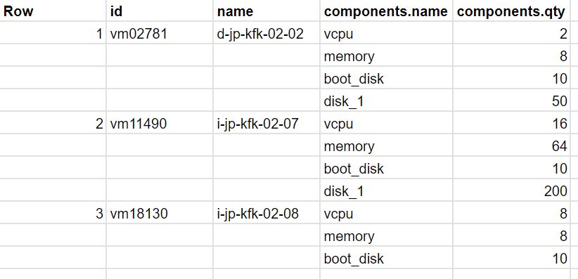
You possess an inventory of VM data stored in a BigQuery table called dataset.inventory_vm. To prepare the data for regular reporting in the most cost-effective manner, you need to exclude VM rows with fewer than 8 vCPUs. What action should you take?
Explanation
Click "Show Answer" to see the explanation here
A. Create a view with a filter to remove rows with fewer than 8 vCPUs, and utilize the UNNEST operator.
Justification:
Create a View: Views in BigQuery are logical queries that act as virtual tables. By creating a view, you can define a filter to exclude VM rows with fewer than 8 vCPUs without modifying the original data. This approach ensures data integrity and allows for easy reuse of the filtered dataset for regular reporting.
Utilize the UNNEST Operator: The UNNEST operator is used to flatten arrays or structs in BigQuery. While it may not be necessary for filtering rows based on vCPUs, it can be useful if the vCPUs data is stored in an array or struct format. If the vCPUs data is stored in a nested structure, you can use UNNEST to access and filter it appropriately.
Option B:
Creating a materialized view with a filter to eliminate rows with fewer than 8 vCPUs is a valid approach. Materialized views store the results of the query in a physical table, which can improve query performance for repeated queries. However, materialized views incur storage costs and may not be necessary for regular reporting unless there's a significant benefit in query performance.
Option C:
Establishing a view with a filter to discard rows with fewer than 8 vCPUs is similar to option A, but it doesn't mention the UNNEST operator. If the vCPUs data is stored in a nested structure, utilizing the UNNEST operator may be necessary to access and filter it correctly.
Option D:
Employing Dataflow to batch process the data and write the result to another BigQuery table is a valid approach but may be overkill for this specific requirement. Dataflow is typically used for more complex data processing tasks or when real-time processing is required. For simple filtering tasks like excluding rows based on a specific condition, using a SQL query and creating a view is a more straightforward and cost-effective solution.
Explanation
A. Create a view with a filter to remove rows with fewer than 8 vCPUs, and utilize the UNNEST operator.
Justification:
Create a View: Views in BigQuery are logical queries that act as virtual tables. By creating a view, you can define a filter to exclude VM rows with fewer than 8 vCPUs without modifying the original data. This approach ensures data integrity and allows for easy reuse of the filtered dataset for regular reporting.
Utilize the UNNEST Operator: The UNNEST operator is used to flatten arrays or structs in BigQuery. While it may not be necessary for filtering rows based on vCPUs, it can be useful if the vCPUs data is stored in an array or struct format. If the vCPUs data is stored in a nested structure, you can use UNNEST to access and filter it appropriately.
Option B:
Creating a materialized view with a filter to eliminate rows with fewer than 8 vCPUs is a valid approach. Materialized views store the results of the query in a physical table, which can improve query performance for repeated queries. However, materialized views incur storage costs and may not be necessary for regular reporting unless there's a significant benefit in query performance.
Option C:
Establishing a view with a filter to discard rows with fewer than 8 vCPUs is similar to option A, but it doesn't mention the UNNEST operator. If the vCPUs data is stored in a nested structure, utilizing the UNNEST operator may be necessary to access and filter it correctly.
Option D:
Employing Dataflow to batch process the data and write the result to another BigQuery table is a valid approach but may be overkill for this specific requirement. Dataflow is typically used for more complex data processing tasks or when real-time processing is required. For simple filtering tasks like excluding rows based on a specific condition, using a SQL query and creating a view is a more straightforward and cost-effective solution.
Question 20 Single Choice
You are overseeing the data lake infrastructure for DataNova Corp, which is built on BigQuery. The data ingestion pipelines pull messages from Pub/Sub and write the incoming data into BigQuery tables. After rolling out a new version of the ingestion pipelines, you notice that the daily data volume stored in BigQuery has surged by 50%, even though the data volume in Pub/Sub hasn't changed. Only certain BigQuery tables show a doubling in the size of their daily partitions.
How should you investigate and resolve the root cause of this increase?
Explanation
Click "Show Answer" to see the explanation here
Correct Answer: C.
1. Check the tables with increased data for duplicated entries.
2. Use BigQuery Audit Logs to trace job activity and retrieve relevant job IDs.
3. Use Cloud Monitoring to identify when each Dataflow job started and determine the associated code version.
4. If multiple pipeline versions are pushing to the same table, stop all except the most recent one.
Justification for Correct Option (C):
This option provides a comprehensive, non-destructive, and systematic approach to:
Investigate the root cause of the data volume spike,
Identify potential duplicate entries,
Trace pipeline behavior via logs, and
Resolve the issue by stopping unintended writes, without risking data loss.
Let’s break it down:
1. Check for duplicated entries
Doubling of partition sizes often indicates duplicate writes. Verifying for duplication is the first logical step.
2. Use BigQuery Audit Logs to trace job activity
BigQuery Audit Logs help identify who or what is writing to a table. They contain:
Job type (e.g., load, query)
Execution timestamp
Service account and job configuration
Relevant docs:
BigQuery Audit Logs
3. Use Cloud Monitoring to identify job start times and versions
Helps correlate pipeline start times with observed anomalies, and determine whether multiple Dataflow jobs (or older versions) are concurrently writing to the same table.
Docs:
Cloud Monitoring for Dataflow
4. Stop unintended concurrent pipelines
If multiple versions of pipelines are found writing to the same sink, stopping the older ones prevents further duplication, resolving the issue at the source.
This diagnoses and remediates the actual issue without reverting or deleting any data.
Why the Other Options Are Incorrect:
Option A:
While checking for duplicates is valid, manually scheduling jobs to clean up duplicates is reactive, not a root cause fix.
Also, this does not explain why duplication started, or prevent recurrence.
Sharing the deduplication script doesn’t help if the pipeline issue persists.
Option B:
Reviewing pipeline code and logging is helpful, but:
No duplication check is mentioned.
Using time travel to restore tables is risky and not recommended as a first step, especially without confirming data corruption.
Time travel only works within 7 days and can be costly if misused.
BigQuery Time Travel
Option D:
Reverting the pipeline and using time travel is drastic.
It does not diagnose the issue, only rolls back.
Reprocessing data via Pub/Sub seek risks data loss or inconsistency, especially if ordering is not guaranteed or deduplication isn’t built in.
Final Answer: C
Explanation
Correct Answer: C.
1. Check the tables with increased data for duplicated entries.
2. Use BigQuery Audit Logs to trace job activity and retrieve relevant job IDs.
3. Use Cloud Monitoring to identify when each Dataflow job started and determine the associated code version.
4. If multiple pipeline versions are pushing to the same table, stop all except the most recent one.
Justification for Correct Option (C):
This option provides a comprehensive, non-destructive, and systematic approach to:
Investigate the root cause of the data volume spike,
Identify potential duplicate entries,
Trace pipeline behavior via logs, and
Resolve the issue by stopping unintended writes, without risking data loss.
Let’s break it down:
1. Check for duplicated entries
Doubling of partition sizes often indicates duplicate writes. Verifying for duplication is the first logical step.
2. Use BigQuery Audit Logs to trace job activity
BigQuery Audit Logs help identify who or what is writing to a table. They contain:
Job type (e.g., load, query)
Execution timestamp
Service account and job configuration
Relevant docs:
BigQuery Audit Logs
3. Use Cloud Monitoring to identify job start times and versions
Helps correlate pipeline start times with observed anomalies, and determine whether multiple Dataflow jobs (or older versions) are concurrently writing to the same table.
Docs:
Cloud Monitoring for Dataflow
4. Stop unintended concurrent pipelines
If multiple versions of pipelines are found writing to the same sink, stopping the older ones prevents further duplication, resolving the issue at the source.
This diagnoses and remediates the actual issue without reverting or deleting any data.
Why the Other Options Are Incorrect:
Option A:
While checking for duplicates is valid, manually scheduling jobs to clean up duplicates is reactive, not a root cause fix.
Also, this does not explain why duplication started, or prevent recurrence.
Sharing the deduplication script doesn’t help if the pipeline issue persists.
Option B:
Reviewing pipeline code and logging is helpful, but:
No duplication check is mentioned.
Using time travel to restore tables is risky and not recommended as a first step, especially without confirming data corruption.
Time travel only works within 7 days and can be costly if misused.
BigQuery Time Travel
Option D:
Reverting the pipeline and using time travel is drastic.
It does not diagnose the issue, only rolls back.
Reprocessing data via Pub/Sub seek risks data loss or inconsistency, especially if ordering is not guaranteed or deduplication isn’t built in.
Final Answer: C